Current transformers (CT) are the eyes of the power system. For protection relays to work correctly during a massive short circuit, the CT must provide an accurate signal without saturating. This is where the 10% error curve comes into play. Overlooking these curves can lead to catastrophic relay failures in high-fault scenarios.

Why Protection Class CT Testing Matters in Real Operations
The hidden risk of CT saturation during faults
In a perfect world, a CT would scale down primary current to secondary current with zero loss. In reality, some current is always lost to magnetize the core. During a heavy fault, if the primary current is many times the rated value, the CT may saturate. This causes the secondary current to drop significantly, leading to protection relay failure.
Technical Foundations: From Equivalent Circuits to Excitation

Analyzing the CT equivalent circuit model
To understand error, we must look at the CT equivalent circuit. The primary current (Ip) is converted to the secondary side (I2), but it splits into two paths. One part is the excitation current (Ie) flowing through the excitation impedance (Ze), while the other part (Is) flows into the external burden (Zb).
Why excitation current is the root cause of error
The excitation current (Ie) represents internal losses like magnetic and eddy currents. Because Ie consumes a portion of the transformed current, the Is we measure externally is always slightly less than the ideal I2. Since excitation impedance (Ze) changes with the induced electromotive force (Es), we must measure the excitation characteristic curve to understand this relationship.
Step-by-Step Calculation for the 10% Error Curve
Measuring winding resistance and excitation characteristics
First, we measure the secondary winding DC resistance (Rct) and calculate the winding impedance (Z2 = Rct + jXct). Then, we perform an excitation test to plot the U = f(Ie) relationship curve.
Deriving the relationship between K_ALF and secondary burden
The 10% Error Curve: Similarly, this defines the maximum allowable secondary burden for various K_ALF values while ensuring the composite error does not exceed 10%.

The 5% Error Curve: This curve establishes the relationship between the Accuracy Limit Factor (K_ALF)—the ratio of primary current to rated primary current—and the allowable secondary burden when the current error is exactly 5%.

Drawing the error curve involves several logical steps:
Set the Error Limit: For a 10% error, we define the total secondary current as 10 times the excitation current (I2 = 10 * Ie).
Calculate Secondary Output: Using the circuit model, Is = I2 - Ie, which results in Is = 9 * Ie.
Determine K_ALF: The Accuracy Limit Factor (K_ALF) is the ratio of primary current to rated primary current. For a CT with a 1A secondary rating, K_ALF = 10 * Ie.
Map to Allowable Burden: For each K_ALF value, we find the corresponding voltage (U) on the excitation curve and calculate the allowable burden (Z) using the formula Es / Is - Z2.
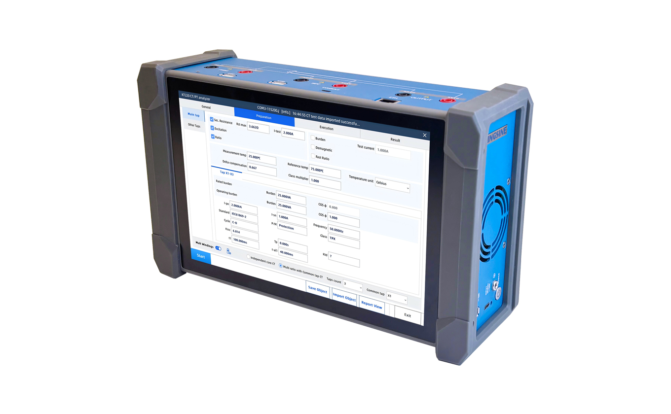
Simplifying Field Work with the KT220 Current Transformer Analyzer
Modern tools like the KINGSINE KT220 Current Transformer Analyzer automate this complex math. While traditional methods require heavy equipment, the KT220 uses advanced frequency-conversion to test excitation characteristics efficiently. It automatically generates 5% and 10% error curves, mapping the relationship between K_ALF and the allowable load in VA or Ohms.
KINGSINE provides this high-precision technology at a much more accessible investment level than many European brands. This allows utilities to equip more field teams with 0.05% accuracy tools without breaking the budget.
FAQs on CT Error Curves and Standards
What is the difference between a 5% and 10% error curve?
Both curves show the relationship between the primary current multiple and the maximum secondary burden. The 5% curve is stricter for high-precision protection, while the 10% curve is standard for most general protection.
How does burden affect the error?
Higher burden increases the voltage the CT must produce. This pushes the CT core toward saturation, increasing excitation current and overall error.
Can I use the KT220 for both CT and VT testing?
Yes, the KT220 is a comprehensive analyzer for both Current Transformers (CT) and Voltage Transformers (VT).


